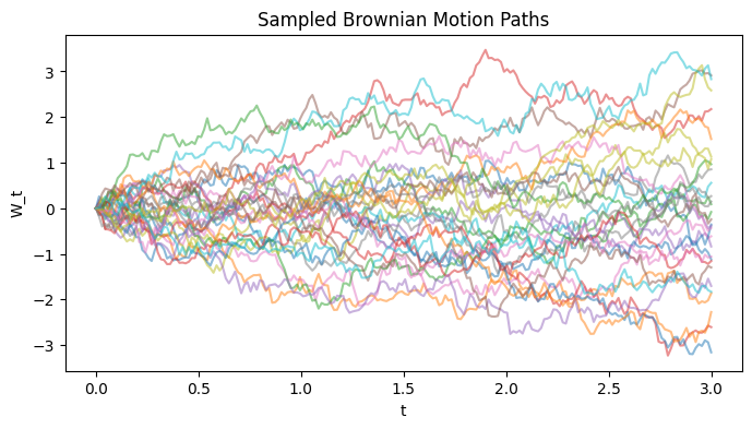
Consider a fixed Brownian motion path \(\{W_t\}_{t \ge 0}\) that we have made observations \(\{W_n\}_n\) at times \(\{t_n\}_n\), we wish to upscale the observed path to more timestamps \(\{s_m\}_m\) while making sure that it is the same Brownian motion path that we are simulating from.
By definition, a Brownian motion has Gaussian increments \(W_{t+u} - W_t \sim N(0, u)\) and the increments are independent of past values \(W_s\) for \(s < t\). It is straightforward also to view a Brownian motion as a Gaussian process (GP) with mean zero and kernel \(k_\text{BM}(W_s, W_t) = \min\{s, t\}\).
Leveraging this GP interpretation, the task of “upscaling” or “extrapolating” given observations of a Brownian path \(\{W_n\}_n\) to additional timestamps \(\{s_m\}_m\) would be equivalent to finding the posterior predictive distribution at the additional timestamps \(\{s_m\}_m\) where we condition on exact observations \(\{W_n\}_n\). In particular, to find \(\{W_{s_m}\}_m\), we can simply find the posterior predictive, then sample from it.
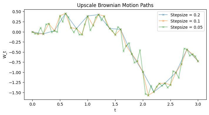
To be fair, this is quite inefficient and I am not sure if there would be any use case for this particular way of upscaling Brownian paths. My original motivation was to simulate coupled Brownian paths for multilevel Monte Carlo layers, but for in such cases we could simply sample a Brownian path with the two timestamps aggregated i.e. \(\{t_n\}_n \cup \{s_m\}_m\) and pick out the needed portions – the order won’t matter there. Doing this GP posterior predictive approach is much more computationally costly for obvious GP reasons, but oh well, thought this at least feels cool.
The Python code is here.