Probabilistic numeric aim to recast numerical algorithms probabilistically to provide uncertainty quantification to the algorithm outputs. Here, we look at how to turn ODE solvers probabilistic.
Consider the generic initial value problem, consisting an ODE between \([0, T]\) with boundary condition
\[ \frac{d}{dt} y(t) = f(y(t), t) \qquad y(0) = y_0 \in \mathbb{R}^d \]
where \(f\) is a (potentially nonlinear) function indicating the drift of the dynamics, where we aim to obtain a solution (function) \(y:[0,T] \to \mathbb{R}^d\) satisfying the above conditions. Now, solving such problems exactly could be difficult, so one often solve them approximately using numerical methods. We often denote the true solution as \(y\) and the approximate solution as \(x\).
We can first rephrase the problem into the residual form
\[ \frac{d}{dt} y(t) - f(y(t), t) = 0 \]
and the collocation method (one class of ODE solvers) aims to make sure the solution \(x\) matches the above residual equation at multiple collocation points, i.e. we consider time steps \(t_1, t_2, \ldots, t_k\) such that
\[ z(t_n) := \frac{d}{dt} x(t_n) - f(x(t_n), t_n) = 0 \quad \forall n. \]
This collocation method1 is the key to the probabilistic solver we will be discussing below.
Probabilistic ODE Solver
The probabilistic solver establishes a Bayesian inference framework where we use the ODE conditions (dynamics and boundary conditions) as data to update our belief of the solution function.
Prior
For the first-order2 ODE we are considering here, we consider the following prior two-dimensional stochastic process \(\{X_t\}\) satisfying the SDE
\[ dX_t = d\begin{bmatrix} X_t^{(1)} \\ X_t^{(2)} \end{bmatrix} = [F X_t + u] dt + L dB_t \]
where \(F, u, L\) are known constant matrices. Here, \(X_t^{(1)}\) denotes the solution function and \(X_t^{(2)}\) denotes the first derivative of the solution function – this requires the constant matrices of the above SDE to satisfy
\[ dX_t^{(1)} = X_t^{(2)} dt \]
for any \(t\).
The precise prior choices (i.e. the choices of \(F, u, L\)) include a \(\nu\)-times integrated Wiener process (IWP(\(\nu\))), a \(\nu\)-times integrated Ornstein-Uhlenbeck process, or a Mat'ern process of order \(\nu + 1/2\). We also remark here that the SDE is linear, thus the transition can be obtained exactly following standard stochastic calculus results.
Data
As mentioned earlier, the data here are the collocation residuals. We define the residual dynamics
\[ Z_t := X_t^{(2)} - f(X_t^{(1)}, t) =: \dot{C} X_t - f(C X_t , t) \]
where we create constant matrices \(C, \dot{C}\) that selects the correct coordinates (original solution and its first derivatve) of the full dynamics \(\{X_t\}\).
The data are thus zero-values of \(Z_t\) at selected time steps \(t_1, t_2, \ldots\). For simplicity, we consider fixed stepsize \(h\) so \(t_{n+1} = t_n + h\) and write \(Z_n := Z_{t_n}\) to make the notation neater. Therefore, our data / observations are the collocation points, as well as the initial conditions
\[ Z_1, Z_2, \ldots, Z_k = 0, \quad CX_0 = y_0. \]
Posterior
To construct the posterior dynamics – which is also the ODE solutions – we just need to assimilate the data into the prior dynamics. Notice that the prior dynamics is driven by a linear SDE, the assimilation can be obtained via a standard Kalman filter and smoother if the data are linearly dependent on the dynamics.
Unfortunately, we are often interested in nonlinear ODEs, which means \(f\), and therefore \(Z\), would be nonlinear, thus requiring either linearization (extended Kalman filter) or particle approximation (particle filter).
Below, we first present the general posterior update. In subsequent subsections, the extended Kalamn filter (EKF) approximations will be described. The particle filter approach would not be covered here.
First, at uniform, discrete time steps \(t_1, t_2, \ldots, t_k\) with stepsize \(h\), we write \(X_{t_n}\) as \(X_n\) and have the following distributions for all \(n\)
\[ \boxed{ \begin{split} X_{n+1}~|~X_n &\sim N(A_h X_n + \xi_h, Q_h) \\ Z_n ~|~ X_n &\sim N(\dot{C}X_n - f(C X_n, t_n), R) \end{split}} \tag{1}\]
where \(A_h, Q_h, X_h\) are transition matrices directly computable from \(F, u, L\) via integrating the SDE over a time period of \(h\), and \(R\) is the observation noise (could be set to zero).
We write the mean and the covariance of \(X\) at time \(t_n\) as \(\mu_n\) and \(\Sigma_n\) respectively, and use superscripts \(F\) and \(P\) to represent the filtered and propagating distributions respectively. So, we have
\[ \boxed{ \begin{split} X_0 &\sim N(\mu_0^F, \Sigma_0^F) \\ \mu_{n+1}^P &= A_h \mu_{n}^F + \xi_h \\ \Sigma_{n+1}^P &= A_h \Sigma_{n+1}^F A_h^T + Q_h \end{split}} \]
for the propagating mean and covariance, and
\[ \boxed{ \begin{split} S_n &= \text{Var}[\dot{C}X_n - f(CX_n, t_n) ~|~ Z_{1:n-1}] + R \\ K_n &= \text{Cov}[X_n, \dot{C}X_n - f(CX_n, t_n) ~|~ Z_{1:n-1}] S_n^{-1} \\ \hat{z}_n &= \mathbb{E}[\dot{C}X_n - f(CX_n, t_n) ~|~ Z_{1:n-1}] \\ \mu_n^F &= \mu_n^P + K_n (z_n - \hat{z}_n) \\ \Sigma_n^F &= \Sigma_n^P - K_n S_n K_n^T \end{split}} \tag{2}\]
for the filtered mean and covariance. Again, it can be noticed that the linearity of (or lack there of) \(f\) determines if the updates are analytic or not.
Finally, we will conduct the backward pass of smoothing. The commonly used Rauch-Tung-Striebel (RTS) smoother is provided by
\[ \boxed{ \begin{split} J_n &= \Sigma_n^F A_h^T (\Sigma_{n+1}^P)^{-1}\\ \mu_n^S &= \mu_n^F + J_n (\mu_{n+1}^S - \mu_{n+1}^P) \\ \Sigma_n^S &= \Sigma_n^F + J_n (\Sigma_{n+1}^S - \Sigma_{n+1}^P) J_n^T \end{split}} \]
where we run backwards from \(n = k-1, k-2, \ldots, 0\) and set the final time slice smoothing distribution to be identical to the filtering distribution, i.e. \(\mu_k^S = \mu_k^F\) and \(\Sigma_k^S = \Sigma_k^F\).
Extended Kalman Filter
The extended Kalman filter is an extension of Kalman filter for nonlinear updates by approximating nonlinear updates by a linear proxy via Taylor’s expansion. Here, the key nonlinearity is with \(f(CX_n, t_n)\), which we approximate using either the zeroth-order or the first-order Taylor expansion of \(X_n\) around \(\mu_n^P\), i.e.
\[ f(CX_n, t_n) \approx f(C\mu_n^P, t_n) \quad \text{or} \quad f(CX_n, t_n) \approx f(C\mu_n^P, t_n) + J_f(C\mu_n^P, t_n) C(X_n - \mu_n^P) \]
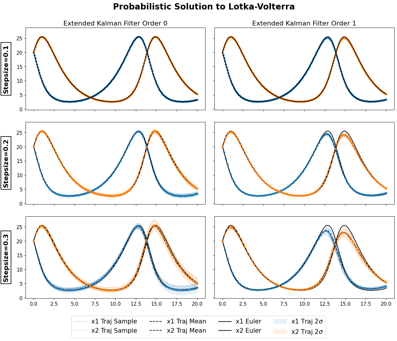
for \(J_f\) being the Jacobian of \(y \mapsto f(y,t)\). The extended Kalman filter thus works by replacing the original \(f\) with the above approximations. The resulting algorithms are termed EK0 and EK1 for zeroth- and first-order approximations respectively.
Example
Solutions to a Lotka-Volterra using EK0 and EK1 against the true solution approximated from an Euler with tiny stepsize. The code can be found here, using the ProbNum python package.